Methods
In this study, we evaluate the effectiveness of data imputation using the LSTM deep learning model during the
data assimilation stage, based on the data of Typhoon MAYSAK (2020). Furthermore, we verify the accuracy
of typhoon track predictions derived from the refined historical data.
I. Data Collection and Preparation
Dataset
Best Track data of the Typhoon occurred between 2016 and 2024 (sourced from data.kma.go.kr)
Variables
Latitude (N), Longitude (E), Central Pressure (hPa), Wind Radius (km), Direction (x and y vectors), and Translation Speed (km/h)
Scenario
Consecutive end-track missing points are intentionally created by deleting specific time-series observation points to simulate the frequent data loss that occurs under realistic circumstances and phenomenon, such as maritime movement.
II. Case Types by Imputation Methods
Case A : Baseline Method (Linear Extrapolation)
Forecast performed using linear extrapolation-imputed observations and a common synthetic background field for EnKF data assimilation.
Step 1: Synthetic Gap Generation
Step 2: Baseline Imputation via Extrapolation
Step 3: Perturbation-based Background Fields
Step 4: Conventional Ensemble Forecasting
Manually generate observation gaps (NaN) within the Typhoon MAYSAK dataset to simulate data loss during maritime movement.
Apply linear extrapolation to restore the missing segments by extending existing trends beyond the last known observation point.
Generate a same synthetic background field by adding artificial perturbations to the true MAYSAK data.
Perform an ensemble simulation using the extrapolated data and perturbed fields to generate the final Maysak trajectory prediction.
Why do we do extrapolation instead of interpolation?
It is the process of estimating an unknown value by extending a known sequence of values beyond the area that is certainly known
The reasons why we chose extrapolation instead of interpolation
Reason 1. A real-time forecasting scenario
Since forecasting is about predicting the future beyond current data, extrapolation is logically required to simulate actual predictive processes.
Reason 2. Simulation of Observation Gaps
We assumed a total loss of data due to equipment failure at sea. Without a future end-point to anchor the data, extrapolation (extending known trends) is the only conventional alternative to interpolation.
Case B : AI-driven Method (LSTM-based Imputation)
Forecast performed using initial conditions derived from LSTM-imputed data and EnKF data assimilation.
Step 1: Deep Learning Model Training
The LSTM model is trained on time-series patterns of typhoon trajectories using historical Best Track data from 2016 to 2024 (excluding MAYSAK).
Step 2: Adaptive Data Imputation & Stress Testing
The pre-trained LSTM model restores missing values in the MAYSAK dataset by leveraging learned temporal patterns. To evaluate robustness, we incrementally increase the missing data ratio to identify the maximum threshold for precise imputation.
Step 3: Perturbation-based Background Fields
Use the same synthetic background field generated from the true MAYSAK data with artificial perturbations. This controlled background field is identical to that used in Case A.
Step 4: Ensemble Forecasting via Integrated Data
Finally, we perform an ensemble simulation by integrating the LSTM-imputed data with the perturbed background fields. This optimizes the initial conditions, allowing for the most reliable and high-accuracy typhoon track predictions.
III. Controlled Background Field Design
To isolate the effect of the imputation method, the same synthetic background field was used in both experiments. The background field was generated by adding artificial errors to the true MAYSAK data.
Formula

Synthetic Background Field
State Variables
The background state vector includes latitude, longitude, central pressure, wind radius, movement direction, and translation speed.


IV. Quantitative Evaluation
We calculate the RMSE (km) for each case to quantitatively determine the percentage by which AI-based data assimilation reduced the forecasting error.
Then we compare the RMSE value to evaluate the performance of two different imputation methods and determine which method outperforms.
Mathematical Framework for Typhoon Track Error Analysis:
1. Coordinate-wise Error Calculation
Determine the squared difference for both Latitude and Longitude independently at each time step (i) to analyze the deviation along each axis.

2. Euclidean Distance Integration
Combine the squared differences to calculate the squared Euclidean distance (di^2), representing the straight-line spatial error between the actual and predicted positions.

3. Quadratic Averaging (MSE)
Compute the Mean Squared Error (MSE) by averaging the squared distances across all n time steps. This process emphasizes and penalizes larger spatial deviations.

4. Final Root Transformation (RMSE)
Apply the square root to the average to derive the Root Mean Square Error (RMSE). This returns the error value to the original coordinate unit (degrees) for intuitive interpretation.

Appendix. Python Codes

Case A Code
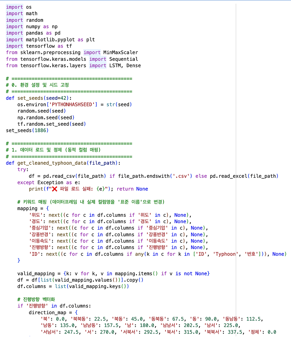
Case B Code